Project Processing
This chapter covers the post-processing workflow for raw scanner data, including project processing, map fusion, and accuracy verification.
Project Processing
Project Processing post-processes raw data from XGRIDS handheld scanners (L2 Pro, K1, K2) to produce the point cloud results you need.
Project Settings
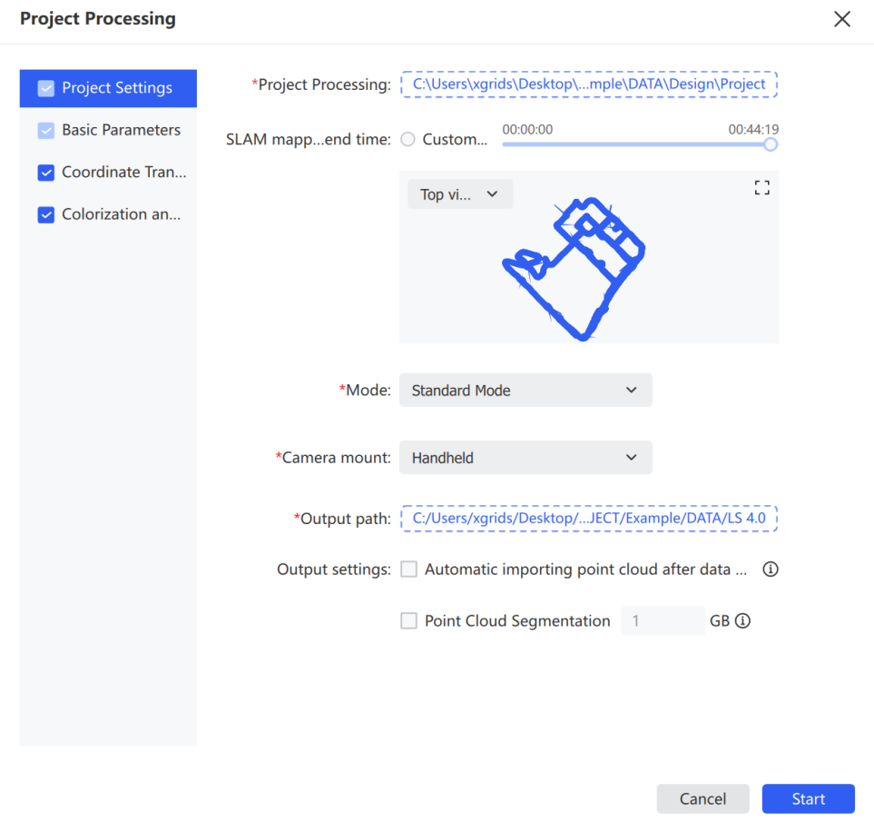
- Click File and select the project data to process. The project path must point to the project directory — the folder copied from the scanning device.
- In Project Processing, confirm the imported data path.
- Set the mapping time range as needed. To limit processing to a specific window, drag the timeline or choose a custom time range.
- Choose a viewing angle in the preview area. Switch between Top, Front, and Left views to inspect the data range and trajectory.
- The preview supports zoom and pan for inspecting project details.
- Choose the mode that matches the project scene.
- Choose the carry method that matches the capture device.
- Set the output path for the processing results.
- Check Auto-load project after processing to load the project automatically once finished.
- Check Point Cloud Segmentation and set the parameter to enable segmentation.
Note: Project Processing supports only XGRIDS handheld scanner data with firmware 2.4.1 or above. Data with firmware between 1.4.0 and 2.4.1 requires Lixel Studio v3.3.1.2; data from firmware earlier than 1.4.0 requires Lixel Studio v2.4.2 or earlier. For L1 devices, firmware 1.4.0 and above requires Lixel Studio v2.5.2.1.
Mode options:
| Mode | Use case |
|---|---|
| Standard | General scenes |
| Robust | Scenes requiring higher processing stability |
| Narrow Space | Tight, structurally constrained environments |
| Vehicle | Vehicle-mounted capture |
| UAV | Drone capture |
Mount method: Handheld, Backpack, Vehicle, UAV.
Basic Parameters
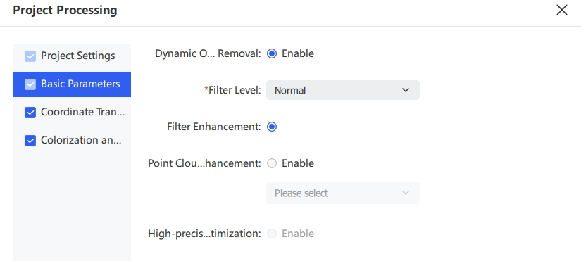
Basic Parameters configures point cloud optimization options during processing — including dynamic object removal, filter enhancement, point cloud enhancement, and high-precision optimization — to improve the quality and usability of results.
- On the Project Processing page, select Basic Parameters in the left panel.
- Adjust the parameters as needed.
| Parameter | Description |
|---|---|
| Dynamic Object Removal | Removes moving objects such as pedestrians or vehicles captured during scanning, improving stability and cleanliness of the result |
| Filter Level | Sets the noise removal intensity. A higher level removes more noise but also more structural detail |
| Filter Enhancement | Further strengthens filtering to reduce the impact of noise and outliers |
| Point Cloud Enhancement | Produces a denser, more uniform point cloud, at the cost of processing efficiency |
| High-Precision Optimization | Further optimizes point cloud quality and detail clarity. Mutually exclusive with Coordinate Transformation |
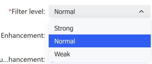
A higher denoising level removes more noise but also more structure. The examples below compare filter levels.
Railing 1 (high density, fully scanned):
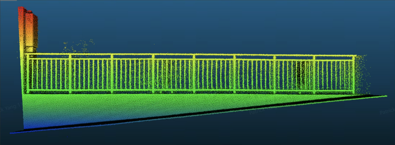
- Strong: More denoising, may remove part of the railing.
- Normal: Balanced denoising, more of the railing intact.
- Weak: Less denoising, minimal damage to the railing.
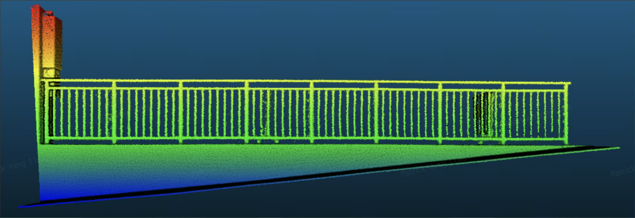
Filter level: Strong
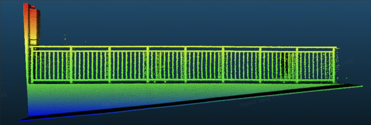
Filter level: Normal
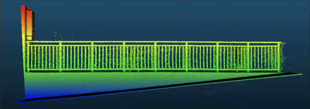
Filter level: Weak
Railing 2 (low density, incomplete scan detail):
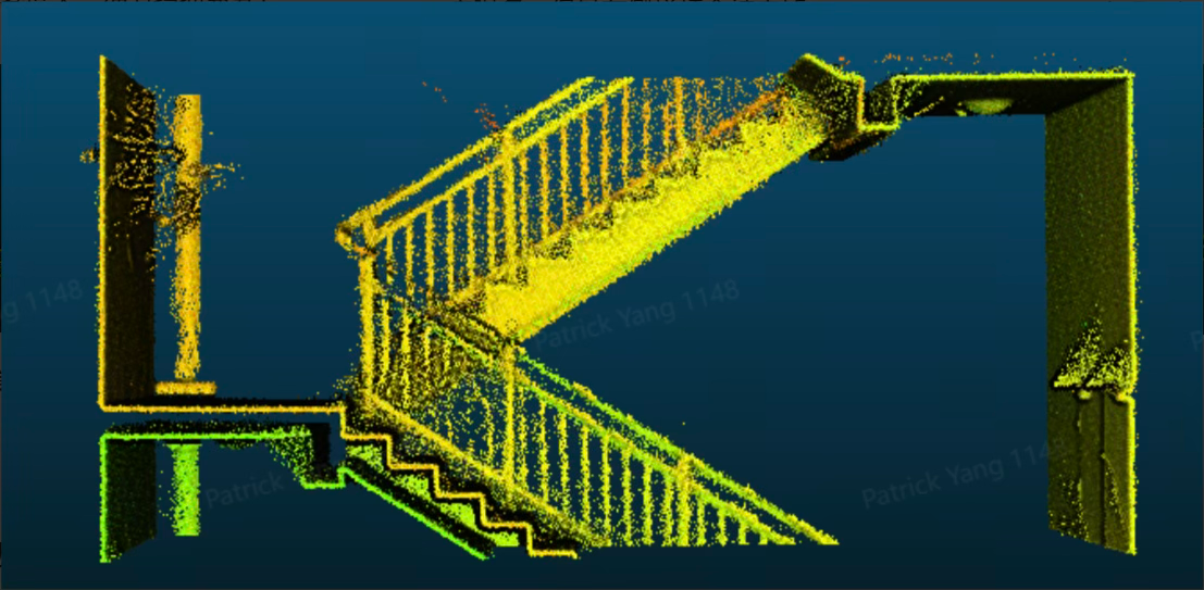
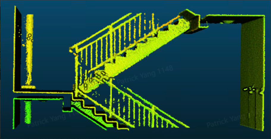
Filter level: Strong
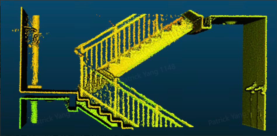
Filter level: Normal
Filter level: Weak
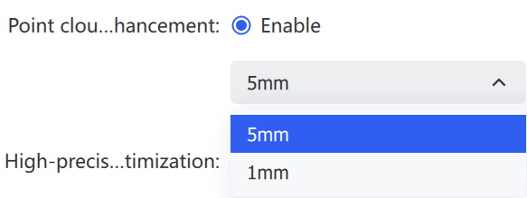
Point Cloud Enhancement: Available in 5mm and 1mm modes for L2 Pro (point spacing ≈ 5mm or 1mm respectively); K1 supports 5mm only. Enabling this reduces processing efficiency and requires adequate hardware, especially for 1mm enhancement which needs sufficient disk space.
Coordinate Transformation
Convert scanned point clouds from the original coordinate system to a target coordinate system. Import a control point file, choose a GNSS data source, set the source and target systems, and complete the transformation through control point matching. Both preset and custom coordinate systems are supported.
- On the Project Processing page, select Coordinate Transformation in the left panel.
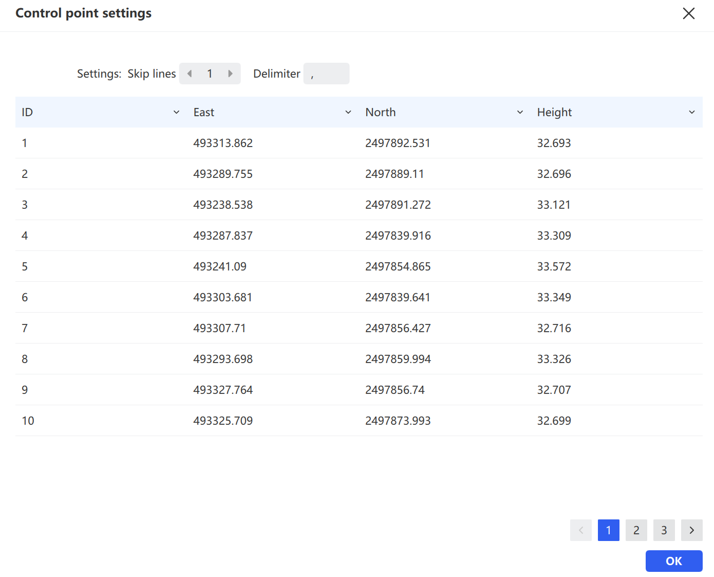
- Import a control point file. Configure Skip Rows and Delimiter as needed. Check GNSS to use GNSS data.
- Choose the GNSS data source — automatic detection from the RTK module, or a GNSS file.
- To match scanned control points with local references, click Edit GCP. In the GCP editor, the left panel shows scanned control points and the right panel shows local reference points. Use the list at the bottom to assign correspondences, then click Confirm to save.
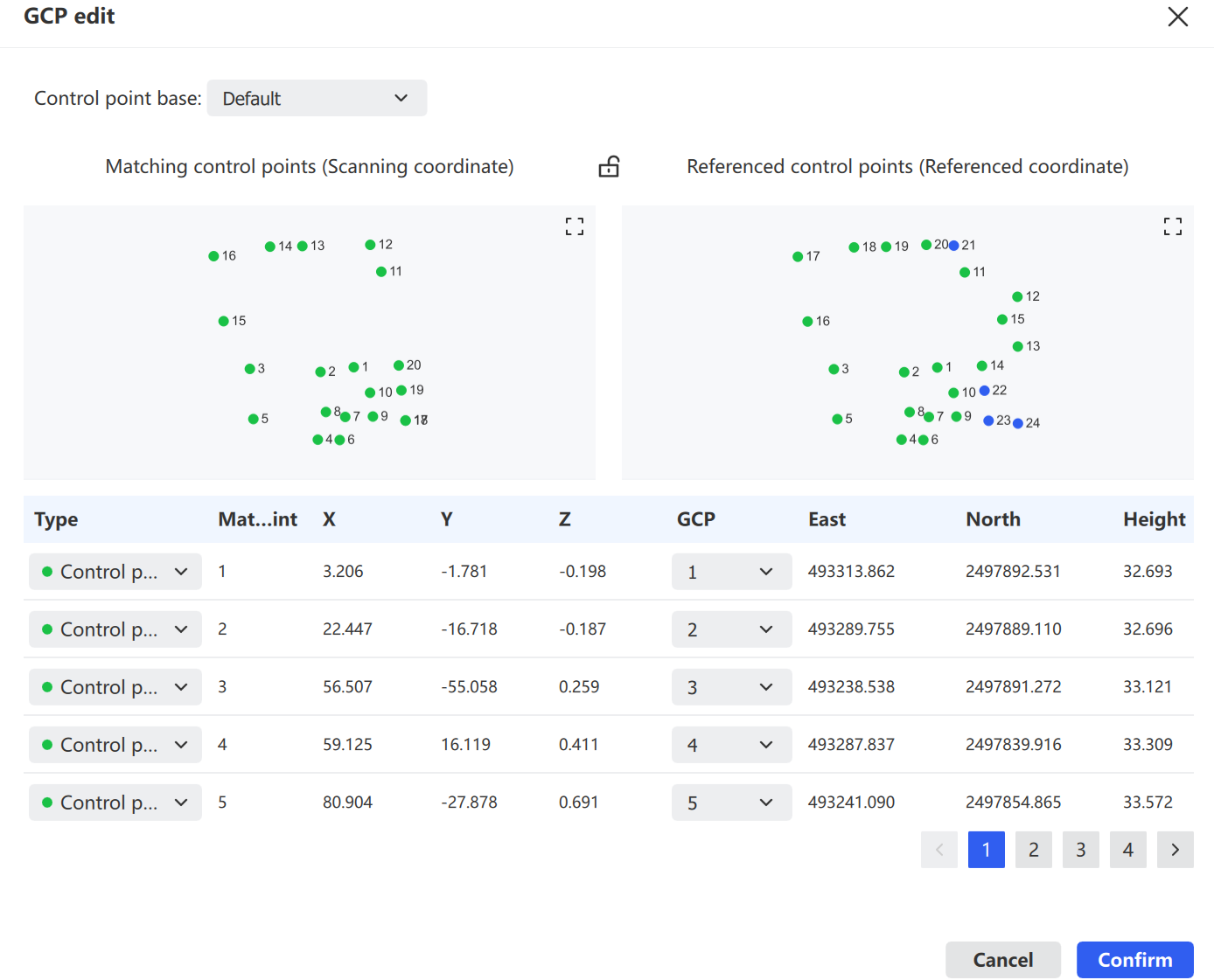
RTK Module: Set Horizontal Accuracy, Satellite Count, and Maximum Tilt, and choose the RTK mount type (Default or Custom).
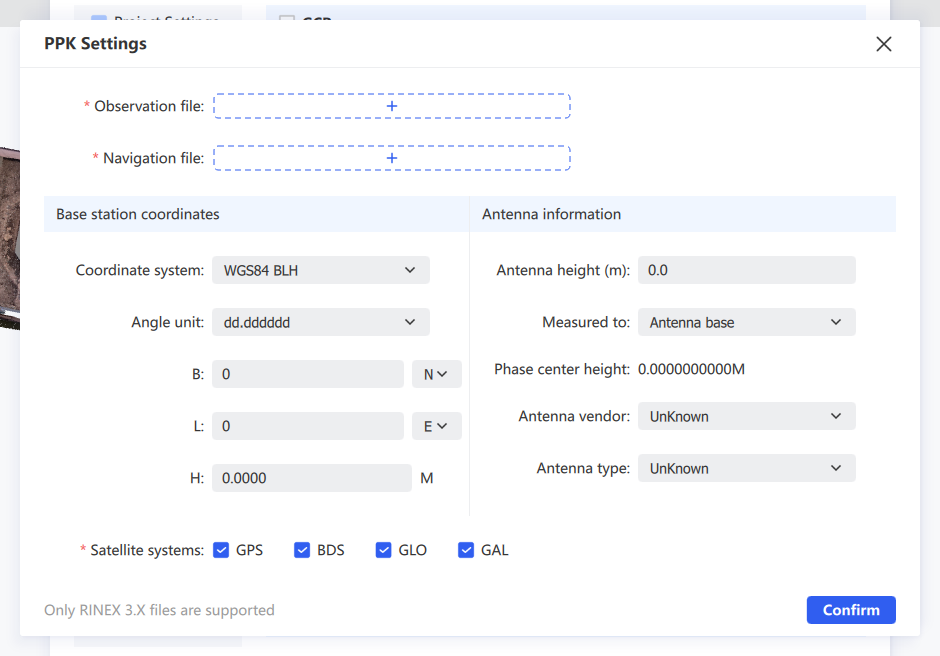
PPK Module: Uses PPK results to enable PPK-SLAM optimization and coordinate transformation when trajectory data is valid. RINEX 3.0 and above only. For data captured in PPK mode, the GNSS module auto-selects PPK during post-processing — click PPK Settings, load the observation and navigation files, adjust base station info, select satellite systems, and click Calculate.
GNSS File: Use third-party software to transform coordinates to a target local system.
- Copy
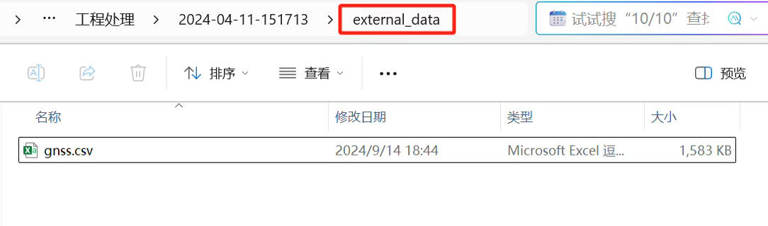
gnss.csvfrom the project's device records.
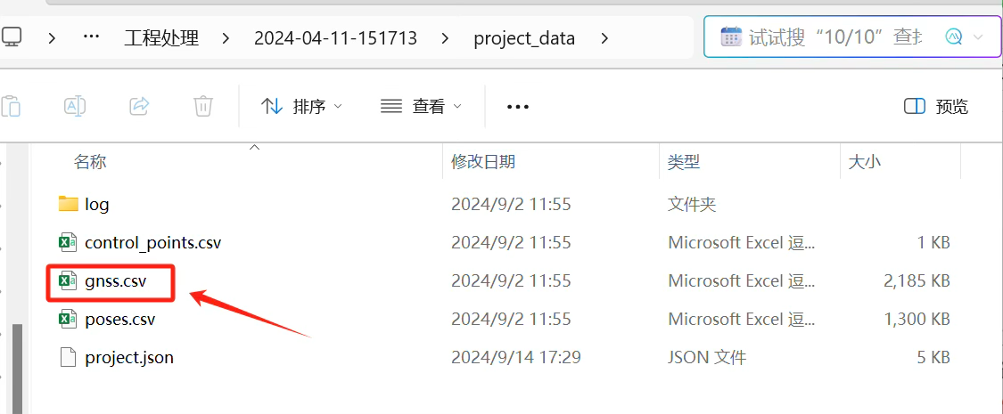
- Transform it in third-party software, then save the result back to the project's
external_datafolder.
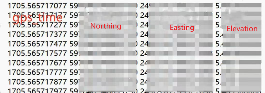
- Check GNSS and select GNSS File. The software reads the file from
external_data. The required format is: gps_time, Northing, Easting, Elevation.
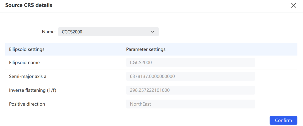
- Review the source coordinate system, and click Details to view its parameters.
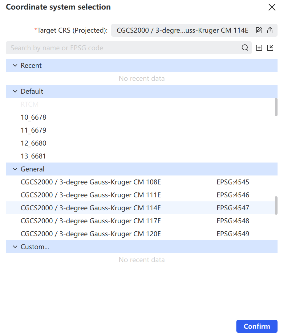
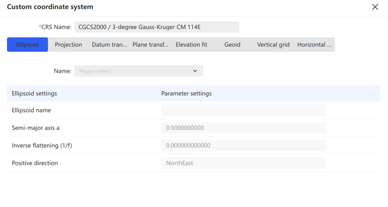
- Click the target coordinate system to open the selector. Choose a preset, or click + to define a custom system (ellipsoid, projection, datum transformation, plane transformation, elevation fitting, geoid, vertical grid, horizontal grid).
- To apply elevation anomaly correction, check Elevation Anomaly and enter a value.
- Click Start to run the transformation, or Cancel to discard.
Coloring and Mesh
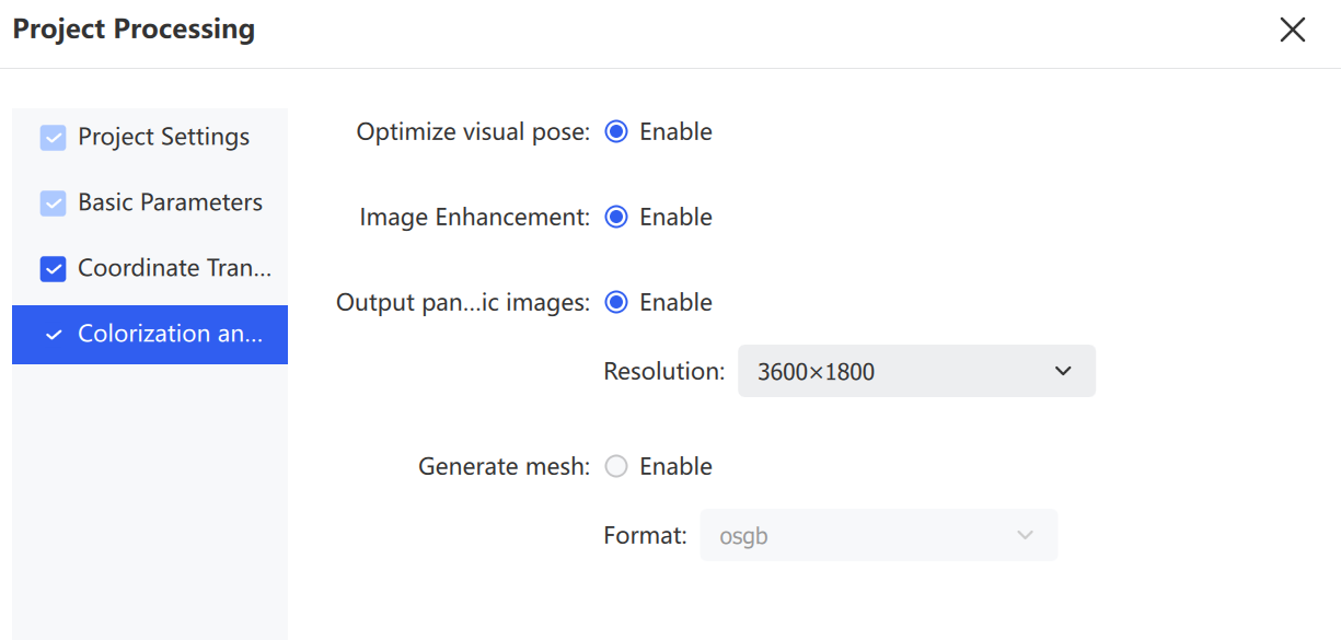
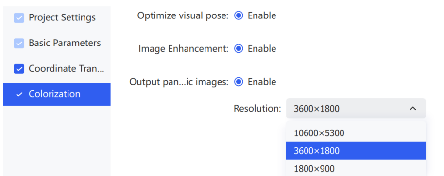
Configures the visual output of project processing results, including optimized visual pose, panoramic image output, and mesh generation with the corresponding resolution and format.
| Parameter | Description |
|---|---|
| Optimize Visual Pose | Improves coloring quality in texture-rich areas |
| Output Panoramic Images | Outputs panoramas alongside the processing results |
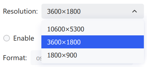
| Resolution | Sets the panorama output resolution |
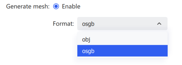
| Generate Mesh | Generates a mesh model, supporting .obj and .osgb formats |
Map Fusion
Map Fusion stitches multiple point cloud datasets into a single map.
For successful fusion, adjacent maps must have a valid connection:
- Adjacent projects must overlap by at least 15m (15–30m recommended). Plan overlaps in feature-rich scenes and avoid open areas, long corridors, and smooth tunnels.
- For RTK-based fusion, RTK data must be valid for every project.
- For fusion based on relative or absolute control points, adjacent maps must share at least one control point with a matching name in the overlap region, and control point names must not be duplicated across projects.
Fusion limitations:
- Up to 10 maps can be fused at once, and each capture session must be under 20 minutes.
- Successfully fused maps are saved as sub-maps in a separate result folder.
- Fusion supports only data from the same device type.
- Use the standard XGRIDS metal control point base when placing control points.
Note: If coordinate transformation is required, all maps must have valid connections (relative control points or continuous scan), and at least 3 absolute control points (not collinear) must exist across all maps.
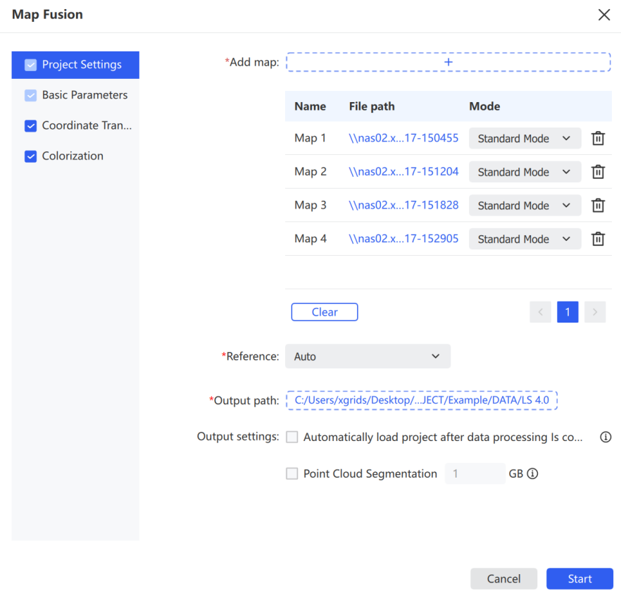
Project Settings
- Click Add Map to import the maps to be fused.
- The list displays each map's point name, file path, and mode.
- Adjust per-map processing in the Mode dropdown.
- Click the trash icon to remove a single map, or Clear to remove all.
- Set the base map — choose Auto or designate one.
- Set the output path.
- Optionally check Auto-load project after processing and Point Cloud Segmentation.
Basic Parameters
Same as Project Processing.
Coordinate Transformation
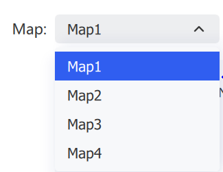
Same as Project Processing. Switch between maps to review.
Coloring
Same as Project Processing.
Accuracy Check
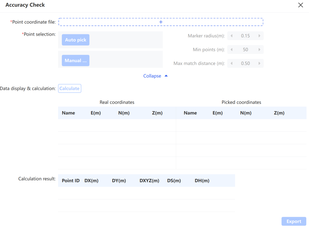
Verify scanned data accuracy by comparing checkpoint coordinates against a set of true values after transformation.
- Select the point cloud data requiring verification, then click Project Processing → Accuracy Check.
- Select checkpoints automatically or manually.
- Review the automatically selected points, and press
Escto exit selection once confirmed correct. - Click Calculate to complete the calculation.
Checkpoint selection in the point cloud
Parameter settings:
| Parameter | Description |
|---|---|
| Point Coordinate File | The true-value coordinate file for checkpoints, in .txt or .csv format: Point Name, Easting, Northing, Ellipsoidal Height (or Point Name, Y, X, Ellipsoidal Height) |
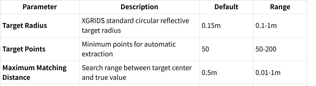
| Target Radius | Radius of the standard circular reflective target, default 0.15m, range 0.1–1m |
| Target Point Count | Minimum number of points required to detect a target during automatic extraction, default 50, range 50–200 |
| Max Matching Distance | Search radius between the target center and the true value, default 0.5m, range 0.01–1m |
Note: Automatic point selection requires XGRIDS reflective targets placed on checkpoints during acquisition. Pause briefly at each target while scanning to ensure enough target points are captured.
Manual point selection: Left-click checkpoint positions in the point cloud (a green label appears). To replace a point, reselect near it and click Yes when prompted. After selecting at least 3 points, press Esc to confirm and exit.
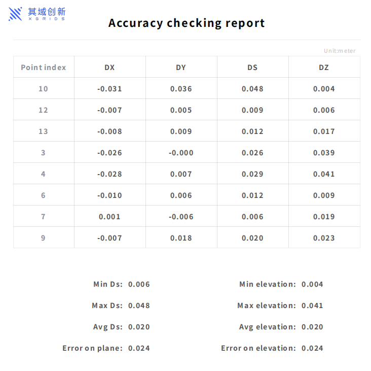
The software then calculates the coordinate differences, planar error, and elevation error (max, min, average) for each point pair, along with the mean square error for plane and elevation. Click Export to save the accuracy report, which defaults to the "Report" folder in the project directory.